Developed a physically-based ray tracing renderer made with C++.

This project began with the goal of simulating realistic lighting in a 3D scene. The major sections of the implementation are as follows:

1. Camera and Ray Generation: creating a virtual camera to cast rays into the scene, allowing us to simulate the process of rendering pixels

2. Ray-Object Intersections: intersection tests to detect when a ray interacts with objects, or primitives, in the scene which allowed us to determine which parts of the scene are visible to the camera

3. Bounding Volume Hierarchy (BVH): To optimize ray-object intersection tests, we use a BVH, which reduces the number of intersection tests by organizing the scene into a hierarchy of bounding volumes, speeding up the rendering process.

4. Direct and Indirect Illumination: simulatation of how light interacts with objects

5. Adaptive Sampling: To reduce noise and speed up rendering, we implemented adaptive sampling, which adjusts the number of samples taken per pixel based on how much noise is present

Together, these components form the foundation of our lighting simulation, allowing for more efficient and realistic rendering in 3D environments.

Camera and Ray Generation

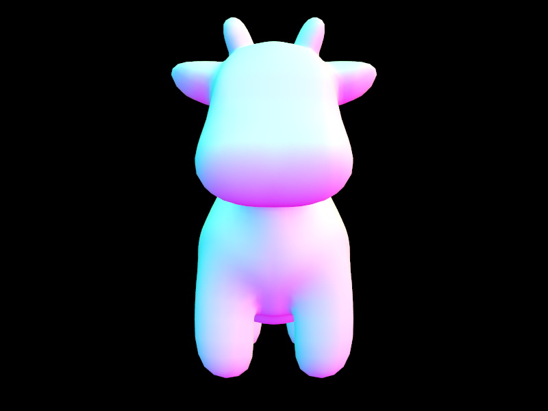
We start by setting up a virtual camera. The virtual camera simulates the viewpoint from which we “see” the scene. It has an origin (basically the camera’s position in 3D space) and a viewing direction (where the camera is pointing). The camera also has a sensor plane, a 2D grid that represents the screen where the final image will be displayed. Each pixel on this sensor plane corresponds to a specific location in the 3D world that the camera is sampling.

To capture a scene, we generate rays that originate from the camera’s position. Each ray passes through the camera’s sensor plane at a specific pixel, and the direction of the ray is calculated based on the camera’s viewpoint and the pixel’s position on the sensor. These rays are used to “sample” the scene, allowing us to gather information about what is visible at each pixel.

Next, we will have to check for rays intersections with objects.

Ray-Object Intersections

At this stage, the process of finding intersections between rays and objects in a scene is done naively. For each ray cast from the camera, we would need to check for intersections with every object in the scene, one by one. This means if there are hundreds or thousands of objects, each ray would require many intersection tests. This is computationally expensive and time-consuming.

For example, in a simple scene with 1,000 objects, a single ray would require 1,000 checks to see if it hits any of the objects. Therefore, we need to optimize this!

This is where Bounding Volume Hierarchy (BVH) comes in. Instead of checking every object individually, BVH organizes objects into a tree structure of bounding volumes (like boxes or spheres) that enclose the objects. This allows us to quickly eliminate large portions of the scene that don’t intersect with the ray, focusing only on the objects within the relevant regions.

Direct Illumination

We start with direct illumination as that is easier to implement. Intuitively, one would do this by tracing rays from the light source to the camera. However, it is more efficient to trace inversely ie rays from the camera to the scene and then determine if those rays reach a light source.

To calculate the pixel color, we check for intersections along these rays and use the irradiance¹ at the intersection point to determine how much light hits it. The pixel’s color is then determined by the light arriving at that point.

For this, we implemented two sampling techniques based on mathematical formulas:

• Uniform hemisphere sampling - where we randomly sample light directions uniformly across the hemisphere around the intersection point.
• Importance sampling - where we focus more on directions that are likely to contribute more light, based on factors like the light source’s intensity and geometry.

Together, these methods allow us to simulate realistic lighting effects by accounting for how light interacts with surfaces and how much of it reaches the camera.

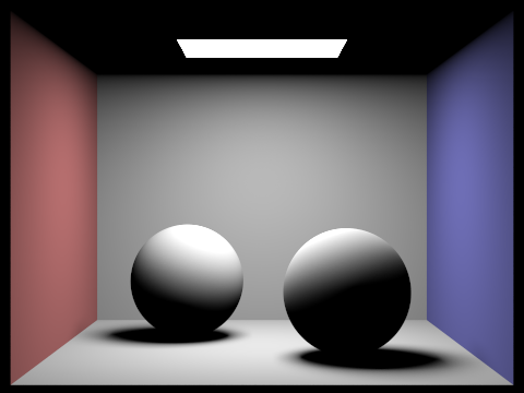Example of a scene rendered with direct illumination

Indirect Illumination

Indirect illumination, or global illumination, is just direct illumination plus the fact that we count additional light bounces. The first light bounce which is when light travels directly from a light source to an object and then to the camera is direct illumination. If the light bounces multiple times instead before reaching the camera, this is indirect illumination. In other words, indirect illumination is direct illumination + additional bounces.

To implement this, we use Monte Carlo sampling, a technique where rays are randomly sampled from the point of intersection to simulate how light bounces around the scene. This randomness helps efficiently estimate the light at a point without checking every possible direction.

After gathering enough samples, we accumulate the results to determine the final pixel color. More bounces result in more realistic lighting although it increases computation time.

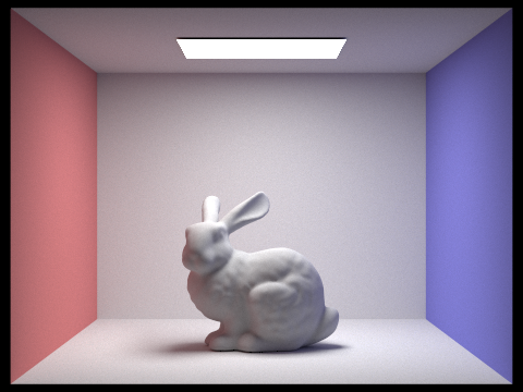
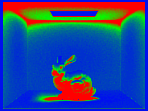
Example of a scene rendered with indirect illumination

Adaptive Sampling

Adaptive sampling optimizes the rendering process by adjusting the number of samples taken per pixel based on the level of noise and complexity in that pixel’s lighting. Since some pixels due to global illumination require more detailed lighting calculations (with more indirect lighting effects), they need more samples to reduce noise while others may require fewer.

To implement adaptive sampling, we evaluate the precision of the pixel’s samples as we collect more. After each group of samples, we calculate the average and variation of the sample values. We then check if the variation is small enough, based on a predefined threshold.

• If the variation is below the threshold, it means the pixel’s samples have stabilized and we can stop sampling early. This avoids unnecessary extra samples, speeding up the rendering process without sacrificing quality.

• If the samples do not converge within the tolerance, the pixel will continue to be sampled up to the maximum limit.

This method ensures that the rendering process is faster, as it allows pixels with stable, low-noise results to stop sampling earlier than others that require more samples.